Acknowledgment

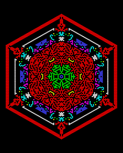
This post owes its existence to a friend of a friend who asked about how the image below was created. This post is my answer to his question.

Of Cellular Automata in General

A picture is worth a thousand words, so I’ll start with an animated picture from a famous cellular automaton:

(Image courtesy of Nathaniel Johnston who has placed it in the public domain.) This animation is a “period 3 oscillator”. The black cells are “alive”, and the white cells are “dead”. At each stage, the cells that are alive in the next generation are governed by the cells that are alive in the present generation. This example comes from John Horton Conway’s Game of Life. The rules that govern which cells become alive and which cells die can be found here.

This is an example of a “square” cellular automaton, and is one of the three regular tilings of the plane, the other two being triangular and hexagonal:

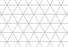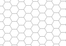Cellular automata are not limited to tilings of the plane, nor are they limited to being organised in any particular or regular pattern. Moreover, there is no requirement for the “life” of any cell to be governed by immediately adjacent cells, nor indeed for the state of any particular cell to be binary. However, for the purposes of study it is convenient to limit oneself to regular tilings of the plane, the cell itself, and immediately adjacent cells, all cells being binary in value.

The Game of Life defines a function from one time step to the next, and has three possible values for every cell in the automaton:

1. Birth
2. Persistence
3. Death

This can be expressed in more mathematical terms as:

1. f(x) = 1
2. f(x) = x (i.e. the identity function)
3. f(x) = 0

The Game of Life uses the values of nine cells (eight adjacent plus the cell itself) when calculating f. Generalising this to the other two regular tilings yields:

	Triangular	Square	Hexagonal
Count	13	9	7

There is also appeal in generalising f as follows:

1. f(x) = 1
2. f(x) = x (i.e. the identity function)
3. f(x) = 1-x (i.e. the inversion, or binary “not”, function)
4. f(x) = 0

For the sake of both clarity and brevity in the rest of this post, it is convenient to use the word “machine”. The machine for the Game of Life looks like this:

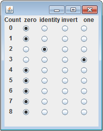
In this scenario, the Game of Life is just one of 4⁹ different machines, and can be notated as “000001I00”. The image at the top of this post is based on 4⁷ different machines, the majority of which turn out to be quite boring. The following comments apply to all machines:

Notation	Observations
000 … 000	All cells are “dead” after the first generation
III … III	Nothing changes
VVV … VVV	Every second generation is the same – the whole automaton merely inverts at every generation
111 … 111	All cells are “alive” after the first generation

Some cellular automata result in an ever growing number of “live” cells. The example below is from the Game of Life. It was made by Kieff, and is reproduced under a CC BY-SA 3.0 licence:

Of Some Particular Hexagonal Cellular Automata

The machines used in the creation of the image at the top of this post started with the following question: “If I start with a single live cell, what happens to it under the complete range of machines?”. It turns that some of them grow forever. The first 17 generations of machine “0000I10” look like this:

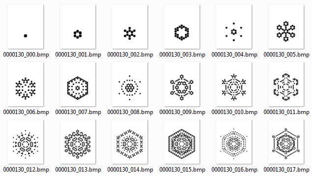
The natural extension of this idea is “What do successive (and not ‘boring’) machines look like at the same generation?”, to which this is a typical answer at generation 13:

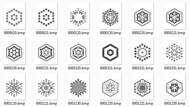
and you can see machine 0000I10 at generation 13 (filename 0000130.bmp) in both images.

(As an aside, the folder in my computer that contains the generation 13 images has a total of 2,282 files and is 13.3 GB in size.)

Monochrome is all well and good, but adding colour adds visual interest. The easiest way to do this is to take successive triples of images, assign each member of a triple to red, green and blue channels, and combine the result:

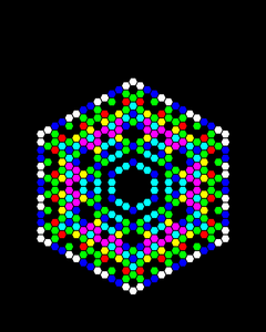
The image immediately above is composed as follows:

Channel	Machine
red	0000IV0 (0000120)
green	0000I10 (0000130)
blue	0000VV0 (0000220)

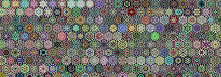
The final step was to arrange the composite hexagons into the image at the top of this post.

And by way of a bonus image, here is machine 000I11I at generation 50 coloured using a completely different algorithm: